R packages
R packages
Data package: edbuildr
Mapping package: edbuildmapr
EdBuild Data Resources
Master Data
codebook = master_codebook()| Variable.Name | Description | Data.Source |
|---|---|---|
| State | State Name | F33 |
| STATE_FIPS | ANSI/FIPS State Code | F33 |
| CONUM | County Code | F33 |
| NCESID | Agency ID - NCES Assigned | NCES |
| Name | School System Name | F33 |
| ENROLL | Fall Membership | F33 |
| SLR | Total Revenue from State and Local Sources | F33/EdBuild |
| SR | Total Revenue from State Sources | F33/EdBuild |
| LR | Total Revenue from Local Sources | F33/EdBuild |
| SLRPP | Total Revenue from State and Local Sources Per Pupil | F33/EdBuild |
| SRPP | Total Revenue from State Sources Per Pupil | F33/EdBuild |
| LRPP | Total Revenue from Local Sources Per Pupil | F33/EdBuild |
| SLRPP_cola | Total Revenue from State and Local Sources Per Pupil Cost-adjusted | F33/C2ER/EdBuild |
| SRPP_cola | Total Revenue from State Sources Per Pupil Cost-adjusted | F33/C2ER/EdBuild |
| LRPP_cola | Total Revenue from Local Sources Per Pupil Cost-adjusted | F33/C2ER/EdBuild |
| County | County Name | NCES |
| state_id | State Agency ID for District | NCES |
| dType | Local Educaion Agency Type | NCES |
| dUrbanicity | Locale, Urban-Centric | NCES |
| dOperational_schools | Total Number Operational Schools | NCES |
| dEnroll_district | Total Students, All Grades (Excludes AE) | NCES |
| FRL | Free and Reduced Lunch Students | NCES |
| FRL_rate | Percent of Free and Reduced Lunch Students | NCES/EdBuild |
| LEP | Limited English Proficient (LEP) / English Language Learners (ELL) | NCES |
| IEP | Individualized Education Program Students | NCES |
| dWhite | White Students | NCES |
| pctNonwhite | Nonwhite Enrollment | NCES |
| dBlack | Black Students | NCES |
| dHispanic | Hispanic Students | NCES |
| dHawaiian_PI | Hawaiian Nat./Pacific Isl. Students | NCES |
| dAsian_PI | Asian or Asian/Pacific Islander Students | NCES |
| dAmIndian_Aknative | American Indian/Alaska Native Students | NCES |
| d2plus_races | Two or More Races Students | NCES |
| Tpop | Estimated Total Population | SAIPE |
| StPop | Estimated Population age 5-17 | SAIPE |
| StPov | Estimated number of relevant children 5 to 17 years old in poverty who are related to the householder | SAIPE |
| StPovRate | StPov/StPop | SAIPE |
| MHI | Median Household Income | EDGE, ACS 5-year |
| MPV | Median Owner-Occupied Property Value | EDGE, ACS 5-year |
| sd_area | Area (square miles) | EdBuild |
| students_per_sq_mile | Students per square mile | EdBuild/NCES |
Taming the System: Common Data Questions... and Answers!
library(openxlsx)
library(ggplot2)
library(scales)
library(knitr)


master17 <- masterpull(data_year = "2017", data_type = "geo")

### this file was downloaded from https://apps.dese.mo.gov/MCDS/home.aspx
### Current Expenditure Per ADA 2009-10 to 2017-18
mo_ada <- read.xlsx("/MO_ADA.xlsx", sheet = "2016-2017") %>%
  select(District.Code, ADA) %>%
  mutate(state_id = gsub("-", "", District.Code))

st_louis_county <- master17 %>%
  right_join(mo_ada, by = "state_id")%
  filter(CONUM == "29189" | CONUM == "29510") %>%
  select(NAME, ENROLL, ADA, StPovRate, SR) %>%
  mutate(`ADA/Enrollment Ratio` = ADA/ENROLL,
         StateRevper_ADA = SR/ADA,
         StateRevper_Enroll = SR/ENROLL,
         `Miscount Per Student` = StateRevper_ADA - StateRevper_Enroll) %>%
  rename(`Student Poverty Rate` = StPovRate)

st_louis_f <- st_louis_county %>%
  rename(`School District` = NAME) %>%
  arrange(desc(`Student Poverty Rate`)) %>%
  mutate(Enrollment = comma(ENROLL, big.mark = ","),
     ADA = comma(ADA, big.mark = ","),
     `State Revenue Per ADA` = dollar(StateRevper_ADA, accuracy=1, big.mark = ","),
     `State Revenue Per Enrollment` = dollar(StateRevper_Enroll, accuracy=1, big.mark = ","),
     `Miscount of revenue per student` = dollar(`Miscount Per Student`, accuracy=1, big.mark = ","),
     `Student Poverty Rate` = percent(`Student Poverty Rate`, accuracy = 1),
     `ADA/Enrollment Ratio` = percent(`ADA/Enrollment Ratio`, accuracy = 1),
     `State Revenue` = dollar(SR, accuracy=1, big.mark = ",")) %>%
  select(`School District`, `Student Poverty Rate`, Enrollment, ADA, `ADA/Enrollment Ratio`,
     `State Revenue`, `State Revenue Per ADA`, `State Revenue Per Enrollment`,
     `Miscount of revenue per student`)

kable(st_louis_f)| School District | Student Poverty Rate | Enrollment | ADA | ADA/Enrollment Ratio | State Revenue | State Revenue Per ADA | State Revenue Per Enrollment | Miscount of revenue per student |
|---|---|---|---|---|---|---|---|---|
| Normandy Schools Collaborative | 31% | 3,770 | 3,390 | 90% | $28,116,000 | $8,295 | $7,458 | $837 |
| St. Louis City School District | 31% | 28,270 | 21,422 | 76% | $105,949,000 | $4,946 | $3,748 | $1,198 |
| Riverview Gardens School District | 31% | 5,915 | 5,235 | 88% | $38,849,000 | $7,421 | $6,568 | $854 |
| Jennings School District | 29% | 2,570 | 2,369 | 92% | $17,127,000 | $7,229 | $6,664 | $565 |
| Ferguson-Florissant R-II School District | 22% | 10,748 | 9,027 | 84% | $56,426,000 | $6,251 | $5,250 | $1,001 |
| Hancock Place School District | 21% | 1,283 | 1,413 | 110% | $9,514,000 | $6,732 | $7,415 | $-684 |
| Ritenour School District | 20% | 6,485 | 5,687 | 88% | $33,276,000 | $5,851 | $5,131 | $720 |
| Hazelwood School District | 18% | 17,952 | 16,508 | 92% | $90,920,000 | $5,508 | $5,065 | $443 |
| University City School District | 14% | 2,818 | 2,443 | 87% | $14,928,000 | $6,112 | $5,297 | $814 |
| Valley Park School District | 13% | 751 | 824 | 110% | $2,999,000 | $3,638 | $3,993 | $-356 |
| Pattonville R-III School District | 13% | 5,793 | 5,287 | 91% | $24,106,000 | $4,559 | $4,161 | $398 |
| Bayless School District | 13% | 1,571 | 1,640 | 104% | $9,077,000 | $5,535 | $5,778 | $-243 |
| Maplewood-Richmond Heights School District | 10% | 1,366 | 1,194 | 87% | $5,526,000 | $4,628 | $4,045 | $582 |
| Affton 101 School District | 8% | 2,474 | 2,409 | 97% | $8,760,000 | $3,636 | $3,541 | $95 |
| Mehlville R-IX School District | 6% | 10,140 | 9,558 | 94% | $36,377,000 | $3,806 | $3,587 | $219 |
| Brentwood School District | 5% | 676 | 728 | 108% | $3,553,000 | $4,877 | $5,256 | $-379 |
| Lindbergh School District | 4% | 6,677 | 6,116 | 92% | $18,660,000 | $3,051 | $2,795 | $256 |
| Parkway C-2 School District | 4% | 16,603 | 16,752 | 101% | $54,630,000 | $3,261 | $3,290 | $-29 |
| Ladue School District | 4% | 4,063 | 3,832 | 94% | $16,757,000 | $4,373 | $4,124 | $248 |
| Webster Groves School District | 4% | 4,518 | 4,198 | 93% | $18,701,000 | $4,455 | $4,139 | $316 |
| Clayton School District | 3% | 2,254 | 2,455 | 109% | $10,987,000 | $4,475 | $4,874 | $-400 |
| Rockwood R-VI School District | 3% | 19,675 | 19,852 | 101% | $76,819,000 | $3,870 | $3,904 | $-35 |
| Kirkwood R-VII School District | 3% | 5,780 | 5,263 | 91% | $18,844,000 | $3,580 | $3,260 | $320 |
stlouis <- ggplot(st_louis_county, aes(`Student Poverty Rate`, `Miscount Per Student`, color = `Student Poverty Rate`)) +
  geom_point(mapping = aes(size = ENROLL)) +
  scale_color_gradient(low="#dff3fe", high="#19596d") +
  theme_bw() +
  theme(legend.position="none")

Using edbuildr
library(edbuildr)Functions
library(scales)
master_fin = masterpull(data_year = "2017", data_type = "fin")

averages_fin <- master_fin %>%
  summarise(Exclusion = "finance",
             Districts = comma(n()),
            `Average Student Poverty Rate` = percent(mean(StPovRate, na.rm = TRUE), accuracy = 1L),
            `Average Local Rev Per Pupil` = dollar(round(mean(LRPP, na.rm = TRUE), 0)),
`Average Total Rev Per Pupil` = dollar(round(mean(SLRPP, na.rm = TRUE), 0)))| Exclusion | Districts | Average Student Poverty Rate | Average Local Rev Per Pupil | Average Total Rev Per Pupil |
|---|---|---|---|---|
| finance | 13,037 | 17% | $7,308 | $14,413 |
| general | 13,184 | 17% | $7,439 | $14,581 |
| with geography | 13,287 | 17% | $7,457 | $14,601 |
| all districts | 18,381 | 17% | $7,923 | $15,633 |
This function allows you to find the difference between each pair of school district neighbors and calculate the national rank from largest to smallest.
neigh_diff(data_year = "2017", diff_var = "options")## [1] "Percent Difference in Local Revenue Per Pupil"
## [2] "Percent Difference in State Revenue Per Pupil"
## [3] "Percent Difference in Total Revenue Per Pupil"
## [4] "Difference in Local Revenue Per Pupil"
## [5] "Difference in State Revenue Per Pupil"
## [6] "Difference in Total Revenue Per Pupil"
## [7] "Percent Difference in Median Household Income"
## [8] "Percent Difference in Median Property Value"
## [9] "Difference in Median Household Income"
## [10] "Difference in Median Property Value"
## [11] "Percentage Point Difference in Percent Nonwhite Enrollment"
## [12] "Percentage Point Difference in Poverty Rate"
## [13] "Percent Difference in Enrollment, F33"
## [14] "Percent Difference in Local Revenue"
## [15] "Percent Difference in State Revenue"
## [16] "Percent Difference in Total Revenue"
## [17] "Percent Difference in Number of Operational Schools"
## [18] "Percent Difference in Enrollment, CCD"
## [19] "Percent Difference in FRL Students"
## [20] "Difference in Percent FRL"
## [21] "Percent Difference in IEP Students"
## [22] "Percent Difference in LEP Students"
## [23] "Percent Difference in White Enrollment"
## [24] "Percent Difference in Hispanic Enrollment"
## [25] "Percent Difference in Black Enrollment"
## [26] "Percent Difference in Asian Enrollment"
## [27] "Percent Difference in Hawaiian and PI Enrollment"
## [28] "Percent Difference in American Indian and AK Native Enrollment"
## [29] "Percent Difference in Multi-Racial Enrollment"
## [30] "Percent Difference in Total Population"
## [31] "Percent Difference in Student Population"
## [32] "Percent Difference in Students Living in Poverty"
## [33] "Percent Difference in District Area"
## [34] "Percent Difference in Students Per Square Mile"## Please see above for variables you can use to rank neighbors.nabes <- neigh_diff(data_year = "2017", diff_var = "Percentage Point Difference in Percent Nonwhite Enrollment", type = "like")
head(nabes)top10_pnw_nabes <- nabes %>%
filter(`District Enrollment, CCD` > 1000) %>%
select(`Rank_Percentage Point Difference in Percent Nonwhite Enrollment`:`Percentage Point Difference in Percent Nonwhite Enrollment`,`District Percent Nonwhite`, `District Enrollment, CCD`, `Neighbor Enrollment, CCD`) %>%
slice(1:10) %>%
mutate(`Percentage Point Difference in Percent Nonwhite Enrollment` = round2(`Percentage Point Difference in Percent Nonwhite Enrollment`, 2),
`District Percent Nonwhite` = percent(`District Percent Nonwhite`, accuracy = 1L),
`District Enrollment, CCD` = comma(`District Enrollment, CCD`),
`Neighbor Enrollment, CCD` = comma(`Neighbor Enrollment, CCD`))
kable(top10_pnw_nabes)| Rank - Percentage Point Difference in Percent Nonwhite Enrollment | State | District Name | Neighbor Name | Percentage Point Difference in Percent Nonwhite Enrollment | District Percent Nonwhite | District Enrollment, CCD | Neighbor Enrollment, CCD |
|---|---|---|---|---|---|---|---|
| 7 | Alabama | Birmingham City School District | Mountain Brook Schools | 0.95 | 99% | 24,070 | 4,343 |
| 16 | Michigan | Detroit Public Schools Community District | Dearborn City School District | 0.91 | 98% | 45,455 | 20,674 |
| 18 | Arkansas | Pine Bluff Sch Dist 3 | Woodlawn Sch Dist 6 | 0.91 | 99% | 4,070 | 578 |
| 27 | Ohio | Trotwood-Madison City School Dist | Brookville Sch Dist | 0.89 | 94% | 2,581 | 1,415 |
| 28 | Alabama | Birmingham City School District | Walker County School District | 0.89 | 99% | 24,070 | 7,723 |
| 29 | Montana | Browning Elem Sch Dist 9 | West Glacier Elem Sch Dist 8 | 0.89 | 96% | 1,462 | 67 |
| 30 | Ohio | Trotwood-Madison City School Dist | New Lebanon Sch Dist | 0.89 | 94% | 2,581 | 1,163 |
| 35 | Mississippi | Aberdeen School District | Monroe County School District | 0.88 | 97% | 1,298 | 2,358 |
| 37 | New York | Amityville Uf Sch Dist | Massapequa Uf Sch Dist 23 | 0.88 | 95% | 3,150 | 7,083 |
| 39 | New York | Uniondale Uf Sch Dist | Garden City u f Sch Dist | 0.87 | 99% | 7,152 | 3,850 |
bham_neighb <- sd_neighbor_xlsx(school_district = "0100390", table_vars = "options")## Use one or more of the following variables to generate a table:
table_vars = c('Name', 'County', 'Enrollment', 'Poverty Rate', 'Percent Nonwhite', 'Percent FRL',
'Local Revenue PP', 'State Revenue PP', 'Total Revenue PP', 'Median Property Value',
'Median Household Income', 'Type')bham_neighb <- sd_neighbor_xlsx(data_year = "2017", school_district = "0100390", table_vars = c('Name', 'Enrollment', 'Poverty Rate', 'Percent Nonwhite', 'Median Household Income', 'Total Revenue PP', 'Local Revenue PP'))## NOTE:: save your workbook to the desired location using:
openxlsx::saveWorkbook(my_table, file = '~/Documents/neighbor_table.xlsx', overwrite = TRUE)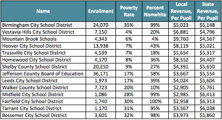
edbuildmapr
Common School District Mapping Questions
What years are school district shapes available?
What's with elementary and secondary districts?
master_shp <- sd_shapepull()

sdType <- as.data.frame(master_shp) %>%
select(-geometry) %>%
group_by(sdType) %>%
summarise(districts = n())
| sdType | districts |
|---|---|
| unified | 10,865 |
| elementary | 1,958 |
| secondary | 486 |
Using edbuildmapr
library(edbuildmapr)Functions
sd17 <- sd_shapepull(data_year = "2017", with_data = TRUE)## Reading layer `shapefile_1718_4269' from data source `/private/var/folders/vz/s7f1ncg12xb6v27z2vzntqjc0000gp/T/RtmpUFwceV/file9c9d5288f72/shapefile_1718_4269.shp' using driver `ESRI Shapefile'
## Simple feature collection with 13330 features and 6 fields
## geometry type: MULTIPOLYGON
## dimension: XY
## bbox: xmin: -179.1686 ymin: 18.91382 xmax: 179.7487 ymax: 71.38881
## epsg (SRID): 4269
## proj4string: +proj=longlat +ellps=GRS80 +towgs84=0,0,0,0,0,0,0 +no_defshead(sd17)ct <- sd17 %>%
filter(State == "Connecticut") %>%
select(urb, StPovRate, LRPP)
plot(ct, border="light gray", lwd=0.5)

ct_map <- sd_map(state="Connecticut", map_var = "Student Poverty")## NOTE::This shapefile has been simplified to make analysis quicker. For final vizualizations, please use the unsimplified shapefiles available through NCES.## NOTE:: save your map to the desired location using: tmap::tmap_save(map, '~/Documents/student_poverty_rate_map.png')ct_map
ct_map_lrpp <- sd_map(state="Connecticut", map_var = "Local Revenue", legend = TRUE)ct_map_lrpp
bham_map <- sd_neighbor_map(school_district = "0100390", map_var = "Percent Nonwhite")bham_map
#### list variables we can use to define neighbors
	borders(diff_var = "options")
## Please see below for variables you can use to define neighbors.## [1] "FIPS" "GEOID" "NAME" "sdType" "State"
## [6] "Postal" "CONUM" "ENROLL" "LRPP" "SRPP"
## [11] "SLRPP" "LR" "SR" "SLR" "COLIn"
## [16] "SRPP_cola" "LRPP_cola" "SLRPP_cola" "County" "dType"
## [21] "urb" "op_shcls" "enroll_ccd" "dFRL" "dLEP"
## [26] "dIEP" "dWhite" "dBlack" "dHispanic" "dAsian_PI"
## [31] "dHaw_PI" "dAmInd_AK" "d2races" "pctNW" "TPop"
## [36] "StPop" "StPov" "StPovRate" "MPV" "MHI"
## [41] "Region" "sd_area" "st_per_sqmi" "year" "frl_rate"neighbors <- borders(shapefile = "2017", id = "GEOID", diff_var = "pctNW", export = "shape") ## this takes 15 minutes to runtop100_pnw_nabes <- neighbors %>%
right_join(nabes, by = "u_id") %>%
filter(`District Enrollment, CCD` > 1000) %>%
slice(1:100)#### adding state shape
states <- st_read("~/Box Sync/Data/Library/SHP/States/States_LowRes_WGS84.shp") %>%
filter(STUSPS != "AK") %>%
filter(STUSPS != "HI") %>%
filter(STUSPS != "PR")map <- tmap::tm_shape(states) +
tmap::tm_borders(lwd=.75, col = "#3b3b3b", alpha = 1) +
tmap::tm_shape(top100_pnw_nabes) +
tmap::tm_lines(lwd=2, col = "#c90000", alpha = 1) +
tmap::tm_layout(bg.color = NA,
frame = FALSE)
map ### view the map
	#### from CRAN
	install_package("edbuildr")
	install_package("edbuildmapr")

	#### from github
	library(devtools)
	install_github("EdBuild/edbuildr")
	install_github("EdBuild/edbuildmapr")